
The consideration and appreciation of the significance of the concepts of errors
and uncertainties helps to develop skills of inquiry and thinking that are not
only relevant to the group 4 sciences. The evaluation of the reliability of the
data upon which conclusions can be drawn is at the heart of a wider scientific
method, which is explained in section 3 of the “Nature of science” part of the
subject guide. Errors and uncertainties are addressed in “Topic 11: Measurement
and data processing” of the subject guide and this topic can be very effectively
treated through the practical scheme of work.
The treatment of errors and uncertainties is also directly relevant to the
internal assessment criteria of:
·
Exploration (“The methodology is highly appropriate to address
the research question because it takes into consideration all, or nearly all, of
the significant factors that may influence the relevance, reliability and
sufficiency of the collected data.”)
·
Analysis (“The report shows evidence of full and appropriate
consideration of the impact of measurement uncertainty on the analysis.”)
·
Evaluation (“Strengths and weaknesses of the investigation, such
as limitations of the data and sources of error, are discussed and provide
evidence of a clear understanding of the methodological issues involved in
establishing the conclusion.”)
The expectations with respect to errors and uncertainties in internal assessment
are the same for both standard and higher level students and are supported by
topic 11 of the subject guide.
Within practical work, students should be able to:
·
design procedures that allow for relevant data to
be collected, in which systematic errors are minimized and random errors are
reduced through the choice of appropriate techniques and measuring instruments,
and by incorporating sufficient repeated measurement where appropriate
·
make a quantitative record of uncertainty range
·
state the results of calculations to the
appropriate number of significant figures. The number of significant figures in
any answer should reflect the number of significant figures in the given data
·
propagate uncertainties through a calculation so
as to determine the uncertainties in calculated results and state them as
absolute and/or percentage uncertainties. Only a simple treatment is required.
For functions such as addition and subtraction, absolute uncertainties can be
added; for multiplication, division and powers, percentage uncertainties can be
added. If one uncertainty is much larger than the others, the approximate
uncertainty in the calculated result can be taken as due to that quantity alone
·
determine from graphs, physical quantities (with
units) by measuring and interpreting a slope (gradient) or intercept. When
constructing graphs from experimental data, students should make an appropriate
choice of axes and scale, and the plotting of points should be clear and
accurate. (Millimetre-square graph paper or software is appropriate.
Quantitative measurements should not be made from sketch graphs.) The
uncertainty requirement can be satisfied by drawing best-fit curves or straight
lines through data points on the graph. (Note: Chemistry students are not
expected to construct error bars on their graphs. However, students, probably
those who also study IB physics, often construct error bars and there is no
requirement to discourage them from doing so.)
·
justify their conclusion by discussing whether
systematic errors or further random errors were encountered. The direction of
any systematic errors should be appreciated. The percentage error should be
compared with the total estimated random error as derived from the propagation
of uncertainties
·
comment on the precision and accuracy of
measurements when evaluating their procedure
·
suggest how the effects of random uncertainties
may be reduced and systematic errors eliminated. Students should be aware that
random, but not systematic, errors are reduced by taking repeated readings.
Systematic errors arise from a problem in the experimental
set-up that results in the measured values always deviating from the “true”
value in the same direction—that is, always higher or always lower. Examples of
causes of systematic error are miscalibration of a measuring device or poor
insulation in calorimetry experiments.
Random errors arise from the imprecision of measurements and
can lead to readings being above or below the “true” value. Random errors can be
reduced with the use of more precise measuring equipment or their effect can be
minimized through repeating measurements so that the random errors cancel out.
Accuracy is how close a measured value is to the correct value,
whereas precision indicates how many significant figures there
are in a measurement. For example, a mercury thermometer could measure the
normal boiling temperature of water as 99.5°C (± 0.5° C), whereas a data probe
may record it as 98.15°C (± 0.05°C). In this case, the mercury thermometer is
more accurate, whereas the data probe is more precise. Students should
appreciate the difference between the two concepts (topic 11.1.)
When numerical data is collected, values cannot be determined exactly,
regardless of the nature of the scale or the instrument. If the mass of an
object is determined with a digital balance reading to 0.1 g, the actual value
lies within a range that extends above and below the reading. This range is the
uncertainty of the measurement. If the same object is measured on a balance
reading to 0.001 g, the uncertainty is reduced, but it can never be completely
eliminated. When recording raw data, estimated uncertainties should be indicated
for all measurements.
There are different conventions for recording uncertainties in raw data.
·
The simplest is the least count, which simply
reflects the smallest division of the scale, for example ± 0.01 g on a top-pan
balance.
·
The instrument limit of error: this is usually no
greater than the least count and is often a fraction of the least-count value.
For example, a burette is often read to half of the least-count division. This
would mean that a burette value of 34.1 cm3 becomes
34.10 cm3 (± 0.05 cm3).
Note that the volume value is now cited to one extra decimal place so as to be
consistent with the uncertainty.
·
The estimated uncertainty takes into account the
concepts of least count and instrument limit of error but also, where relevant,
higher levels of uncertainty, as indicated by an instrument manufacturer, or
qualitative considerations such as parallax problems in reading a burette scale,
reaction time in starting and stopping a timer, random fluctuation in a
voltmeter read-out, or difficulties in knowing just when a colour change has
been completed in a rate experiment or titration. Students should do their best
to quantify these observations into the estimated uncertainty.
·
In chemistry internal assessment, it is not
specified which protocol is preferred and a moderator will accept any protocol
in which the recorded uncertainties are of a sensible and consistent magnitude.
Random errors (uncertainties) in raw data feed through a calculation to give an
error in the final calculated result. There is a range of protocols for propagating
errors. A simple protocol is as follows.
·
When adding or subtracting quantities, the
absolute uncertainties are added.
For example, if the initial and final burette readings in a titration each have
an uncertainty of ± 0.05 cm3 then
the propagated uncertainty for the total volume is (± 0.05 cm3)
+ (± 0.05 cm3) = (± 0.1 cm3).
·
When multiplying or dividing quantities, the
percentage (or fractional) uncertainties are added.
For example:
|
molarity of NaOH(aq) = 1.00 M (± 0.05 M) |
percentage uncertainty = [0.05/1.00] × 100 = 5% |
|
volume of NaOH(aq) = 10.0 cm3
(± 0.1 cm3) |
percentage uncertainty = [0.1/10.00] × 100 = 1% |
Therefore, calculated moles of NaOH in solution = 1.00 × [10.00/1000] = 0.0100
moles (± 6%)
The student may convert the calculated total percentage uncertainty back into an
absolute uncertainty or leave it as a percentage.
Note: A common protocol is that the final total percentage uncertainty should be
cited to no more than one significant figure if it is greater than or equal to
2%, and to no more than two significant figures if it is less than 2%.
There are other protocols for combining uncertainties such as “root sum of
square” calculations. These are not required in IB chemistry but are acceptable
if presented by a student.
Repeated measurements can lead to an average value for a
calculated quantity. The final answer may be given using the propagated error of
the component values that make up the average.
For example:
ΔH mean =
[+100 kJ mol–1 (± 10%) + 110 kJ
mol–1 (± 10%) + 108 kJ mol–1 (±
10%)] / 3
ΔH mean =
+106 kJ mol–1 (± 10%)
This is more appropriate than adding the percentage errors to generate 30% since
that would be completely contrary to the purpose of repeating measurements. A
more rigorous method for treating repeated measurements is to calculate standard
deviations and standard errors (the standard deviation divided by the square
root of the number of trials). These statistical techniques are more appropriate
to large-scale studies with many calculated results to average. This is not
common in IB chemistry and is therefore not a requirement in chemistry internal
assessment.
Sample extracts of typical student work from an experiment on volumetric
analysis in acid–base titration are shown in tables 1–3.
|
Final volume / cm3 |
42.5 |
41.5 |
|
Initial volume / cm3 |
2.5 |
1 |
|
Volume of base required / cm3 |
40.0 |
40.5 |
|
Colour of solution at end point |
light pink |
dark pink |
Table 1
Titration of standard NaOH against vinegar
Some appropriate raw data is recorded but there are no uncertainties given and
the number of decimal places is inconsistent. For internal assessment (IA), this
would contribute to a low mark in the analysis criterion.
|
|
Run 1 |
Run 2 |
Run 3 |
|
Initial volume / cm3 (±
0.1 cm3) |
0.0 |
2.7 |
1.0 |
|
Final volume / cm3 (±
0.1 cm3) |
42.2 |
42.7 |
41.5 |
|
Volume of base required / cm3 (±
0.2 cm3) |
42.2 |
40.0 |
40.5 |
Table 2
Titration of standard HCl against NaOH
Some appropriate raw data is recorded with units and uncertainties. However,
relevant qualitative observations are not recorded. For IA, this might
contribute to a mark below the highest level in the analysis criterion.
|
|
Trial 1 |
Trial 2 |
Trial 3 |
|
Initial volume / cm3 |
1.00 |
2.55 |
0.00 |
|
Final volume / cm3 |
42.50 |
43.25 |
40.50 |
|
Total volume of base required / cm3 (±
0.1 cm3) |
41.5 |
40.7 |
40.5 |
Table 3
Titration of 5.00 cm3 vinegar
against the standardized NaOH
Colours of solutions: acid, base and phenolphthalein indicator were all
colourless. At the end point, the rough trial was dark pink. The other two
trials were only slightly pink at the end point.
The student records appropriate qualitative and quantitative raw data, including
units and uncertainties. For IA, this could contribute to the attainment of the
highest level in the analysis criterion.
The following examples of data collection and processing (tables 4–6) are from a
gas law experiment.
|
Temperature T /
°C ± 0.2° C |
Height of column h /
mm ± 0.5 mm |
|
10.5 |
58.0 |
|
20.3 |
60.5 |
|
30.0 |
61.0 |
|
39.9 |
64.0 |
|
50.1 |
64.5 |
|
60.2 |
67.5 |
|
70.7 |
68.0 |
|
80.8 |
71.0 |
|
90.0 |
71.5 |
Table 4
The student designed the data table and correctly recorded the raw data,
including units and uncertainties. For IA, this could contribute to the
attainment of the highest level in the analysis criterion.
|
Temperature (T) |
Height of column (h) |
|
10.5 |
58.0 |
|
20.3 |
60.5 |
|
30.0 |
61.0 |
|
39.9 |
64.0 |
|
50.1 |
64.5 |
|
60.2 |
67.5 |
|
70.7 |
68.0 |
|
80.8 |
71.0 |
|
90.0 |
71.5 |
Table 5
In this table, units and uncertainties are not included. For IA, this could
contribute to a mark below the highest level in the analysis criterion.
|
Temperature |
Height of column |
|
10.5 |
58 |
|
20.3 |
60.5 |
|
30 |
61 |
|
39.9 |
64 |
|
50 |
64.5 |
|
60.2 |
67.5 |
|
70.7 |
68 |
|
80.8 |
71 |
|
90 |
71.5 |
Table 6
Units and uncertainties are not included and the data is recorded in an
inconsistent manner. Significant digits are not appreciated. For IA, this would
contribute to a low mark in the analysis criterion.
Note: In investigations where a very large amount of data is recorded (probably
by a data logger), it may be more appropriate to present the data as a graph.
Any qualitative observations should be recorded as annotations on or below the
graph.
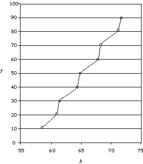
Figures 1 and 2 show graphs of the gas law data from table 4.
Figure 1
Figure 2
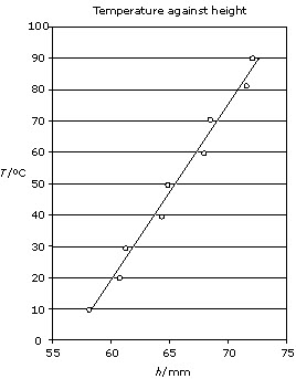
Figure 1 is a graph of the gas law data showing the significant uncertainty. The
computer drew the uncertainty bars based on the assumption that the student had
entered the correct information, which in this case was an uncertainty of 0.5 mm
for each value. Figure 2 does not show the uncertainty bars. In chemistry,
students are not expected to construct uncertainty bars. In
both graphs, the title is given (although it should be more explicit) and the
student has labelled the axes and included units. For IA, this could contribute
to the attainment of the highest level in the analysis criterion.
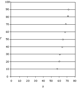
Figure 3

In figure 3, the student does not include a title for the graph and the units
are missing. This would contribute to a low mark in the analysis criterion.
Figure 4
In the examples shown in figure 4, the first student has failed to draw a
best-fit line graph and the second has drawn no line at all. The units and the
titles are missing from the graphs. In the second graph, poor use is made of the
x-axis scale. This would contribute to a low mark in the analysis criterion.
When attempting to measure an already known and accepted value of a physical
quantity, such as the charge on an electron, the melting point of a substance or
the value of the ideal gas constant, students can make two types of comments.
1.
The error in the measurement can be expressed by comparing the experimental
value with the textbook or literature value.
Perhaps a student measured the value of the ideal gas constant, R,
to be 8.11 kPa dm3 mol–1 K–1 and
the accepted value is 8.314 kPa dm3 mol–1 K–1.
The error (a measure of accuracy, not precision) is 2.45% of the accepted value.
This sounds good, but if, in fact, the experimental uncertainty is only 2%,
random errors alone cannot explain the difference and some systematic error(s)
must be present.
2.
The experimental results fail to meet the accepted value (a more
relevant comment).
The experimental range does not include the accepted value: the experimental
value has an uncertainty of only 2%. A critical student would appreciate that he
or she must have missed something here. There must be more uncertainty and/or
errors than have been acknowledged.
In addition to the these two types of comments, students may also comment on
errors in the assumptions of the theory being tested, and errors in the method
and equipment being used. Two typical examples of student work are given in
figures 5 and 6.
Figure 5
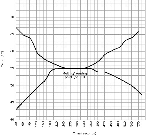
Intermolecular bonds are being broken and formed, which consumes energy.
There is a definite correlation between the melting point and the freezing
point of a substance. If good data is collected, the melting point should be
the same as the freezing point. A substance should melt, go from solid to
liquid, at the same temperature that it freezes, goes from liquid to solid.
Our experiment proved this is true because, while freezing, the freezing
point was found to be 55°C, and when melting, the melting point was also
found to be 55°C (see graph).
The student states a conclusion that has some validity. However, no comparison
is made with the literature value and there is no evaluation of the procedure
and results.
For IA, this would contribute to low marks in the analysis and evaluation
criteria.
Figure 6
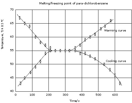
Melting point = freezing point = 55.0 ± 0.5°C
![]()
Literature value of melting point of para-dichlorobenzene = 53.1°C ((Handbook
of Chemistry and Physics, Haynes, W.M. (2012) CRC press).
![]()
The fact that % difference > % uncertainty means random errors alone cannot
explain the difference and some systematic error(s) must be present.
Melting point (or freezing point) is the temperature at which the solid and the
liquid are in equilibrium with each other: (s)
⇌ (l). This is the temperature at which there is no change in kinetic
energy (no change in temperature), but a change in potential energy. The value
suggests a small degree of systematic error in comparison with the literature
value as random errors alone are unable to explain the percentage difference.
Evaluation of procedure and modifications:
Duplicate readings were not taken. Other groups of students had % uncertainty >
% difference, that is, in their case random errors could explain the %
difference, so repeating the investigation is important.
How accurate was the thermometer? It should have been calibrated. In order to
eliminate any systematic errors due to the use of a particular thermometer,
calibration against the boiling point of water (at 1 atmosphere) or better still
against a solid of known melting point (close to the melting point of the
sample) should be done.
The sample in the test tube was not as large as in other groups. Thus the
temperature rises/falls were much faster than for other groups. A greater
quantity of solid, plus use of a more accurate thermometer (not 0.5°C divisions,
but the longer one used by some groups) would have provided more accurate
results.
For IA, this could contribute to the attainment of the highest levels in the
analysis and evaluation criteria.