ERROR ANALYSIS IN BIOLOGY
Error analysis in biology is no different from that in other sciences. Biology however is not an "exact" science in that much of the data collected by biologists is qualitative. Furthermore, biological systems are very complex and difficult to control. Biological investigations, nevertheless, do often require measurements and biologists do need to be aware of the sources of error in their data.
Human error
Obviously data which is carefully recorded will be more reliable than data collected carelessly. Human error can occur when tools or instruments are used or read incorrectly. For example a temperature reading from a thermometer in a liquid should be taken after stirring the liquid and whilst the bulb of the thermometer is still in the liquid. Thermometers and other instruments should be read with the eye level with the liquid otherwise this results in parallax error.
Human errors can be systematic because the experimenter does not know how to use the apparatus properly or they can be random because the power of concentration of the experimenter is fading.
|
|

Systematic errors
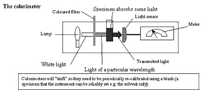
If an electronic water bath is set to 37°C the thermometer in the water bath should also read 37°C. If they do not agree then there will be an error at any other temperature being used. Some instruments need calibrating before you use them. If this is done correctly and regularly it can reduce the risk of systematic error.
Random errors
In biological investigations, the changes in the material used or the conditions in which they are carried out can cause a lot of errors.
For example the rate of respiration of a small animal measured using a manometric respirometer can be influenced by changes in air temperature and barometric pressure.
Biological material is notably variable.
For example, the water potential of potato tissue may be calculated by soaking pieces of tissue in a range of concentrations of sucrose solutions. However, different pieces of tissue will vary in their water potential especially if they have been taken from different potatoes.
The problem of random errors can be kept to a minimum by careful selection of material and careful control of variables (e.g. using a water bath or a blank).
As we saw above, human errors can become random when you have to make a lot of tedious measurements, your concentration span can vary. Automated measuring using a data-logger system can help reduce the likelihood of this error; alternatively you can take a break from measuring from time to time.
|
|
Replicates and samples
Because of their complexity and variability biological systems require replicate observations and multiple samples of material. As rule the lower limit is 5 measurements or a sample size of 5. Very small samples run from 5 to 20, small samples from 20 to 30 and big samples above 30.
Selecting data
Replicates permit you to see if data is consistent. If a reading is very different from the others it may be left out from the processing and analysis. However, you must always be ready to justify why you do this.
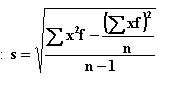
Degrees of precision
If you use a ruler, graduated in millimetres, to measure an object (e.g. the length of a leaf) you will probably find the edges of the object lie close to a millimetre division but probably not right on it. Recording the leaf is "4.5cm-and-a-bit" long is not very useful. The accepted rule is that the degree of precision is ± the smallest division on the instrument, in this case one millimetre. So the leaf in this example is 4.5cm ± 0.1cm.
The degree of precision will influence the instrument that you choose to make a measurement. For example of you used the same ruler to measure an object 0.5cm long the degree of precision (± 0.1cm) is 20% of the measurement, This a is very large error margin and, so, it is not very precise. Therefore, we must choose an appropriate instrument for measuring a particular length, volume, pH, light intensity etc.
The act of measuring
When a measurement is taken this can affect the environment of the experiment. For example when a cold thermometer is put in a test tube of warm water, the water will be cooled by the presence of the thermometer. When the behaviour of animals is being recorded the presence of the experimenter may influence them.
Why bother?
You might think that with all these sources of error and imprecision experimental results are worthless. This is not true, it is understood that experimental results are only estimates. What is expected of a scientist is that they:
- make the best effort to avoid errors in their design of investigations and the use of instruments.
- are aware of the source of errors and to appreciate their magnitude.